Teaching > ECE410F
ECE410F - Linear Control Systems - Fall 2024
Calendar Description
3/1.50m/1m/0.50
III,IV-AECPEBASC, III,IV-AEELEBASC,
I-AEMINRAM
State space analysis of linear systems, the matrix exponential,
linearization of nonlinear systems. Structural properties of linear
systems: stability, controllability, observability, stabilizability,
and detectability. Pole assignment using state feedback, state
estimation using observers, full-order and reduced-order observer
design, design of feedback compensators using the separation
principle, control design for tracking. Control design based on
optimization, linear quadratic optimal control, the algebraic Riccati
equation. Laboratory experiments include computer-aided design using
MATLAB and the control of an inverted pendulum on a cart.
Prerequisite: ECE311H1
Exclusion: ECE557H1
Learning Objectives
In a previous control course you were introduced to the so-called classical control theory, relying on frequency domain methods to design simple feedback loops for single-input single-output linear time-invariant (LTI) control systems. In the 1960s, the field of control systems underwent a revolution, and some say that it became a science. A new way of representing linear time-invariant systems came to the fore, the so-called state-space representation, new problems were formulated, and new tools were developed. This course gives a thorough coverage of the foundational state-space theory of linear control systems. Our progression will be as follows.
- Basic properties: We will review ways to represent LTI control systems, and how to linearize a nonlinear control system about an equilibrium in order to get an LTI model. We will investigate how to predict the qualitative properties of solutions of an LTI system without computing its solutions.
- Stability of LTI systems: The notion of stability is a basic property that we would like an LTI system to possess. In a first control course, you have studied the notion of bounded-input bounded-output (BIBO) stability for LTI systems described by transfer functions. We will port this notion of stability to state-space LTI systems and define new notions of internal stability. We will then develop tests to check whether or not a given LTI system possesses one of these notions of stability.
- Stabilization of equilibria via state feedback: When does there exist a state feedback controller capable of rendering an LTI control system stable? And if such a controller exists, how do we go about designing it? The answer to these questions will take us on a journey through controllability and Kalman decompositions of control systems.
- State estimation: Suppose we have sensors measuring some information about the state of an LTI control system. Under what conditions the sensors contain enough information to reconstruct the entire state? And if such a reconstruction is in principle possible, how do we go about designing a state estimator? We will answer these questions and, using the insight we'll gain in the process, we will learn how to design state estimators, which in control theory are called observers.
- Output feedback stabilization of equilibria: Using state feedback controllers and state estimators, we will design a controller using sensor feedback to stabilize the origin an LTI control system.
- Quadratic optimal control: We will learn how to design a state feedback controller that minimizes the integral over positive time of an instantaneous cost that is quadratic with respect to the state and control vectors. In the process, we will be introduced to the principles of optimal control: dynamic programming and the Hamilton-Jacobi-Bellman (HJB) equation.
- Integral output feedback control: Having learned how to design output feedback controllers stabilizing equilibria, we will learn how to design output feedback controllers tracking constant reference signals while rejecting constant unknown disturbances. These controllers possess integral action.
- Model predictive control (MPC): In quadratic optimal control, we design a controller that minimizes the integral of the instantaneous cost over all positive time. In MPC we wish to design a controller minimizing a cost over a fixed time window that slides forward in time as time progresses. Moreover, in MPC the minimization problem is subject to constraints encoding, for example, actuator saturation or constraints on the state. In this part of the course we will present MPC for LTI systems with quadratic cost and linear state and input constraints.
Instructor
M. Maggiore
Office: GB344
Email address: maggiore (at)
ece.utoronto.ca
Teaching Assistants
| Saima Ali | saiima.ali@mail.utoronto.ca |
| Luiz Dias Navarro | luiz.navarro (at) mail.utoronto.ca |
| Emily Vukovich | emily.vukovich (at) mail.utoronto.ca |
Lectures
| Mon 13-14 | BA1240 |
| Tue 13-14 | BA2165 |
| Thu 14-15 | BA1190 |
Composition of Final Mark
| Labs | 15% |
| Homework Assignments | 5% |
| Midterm 1 | 15% |
| Midterm 2 | 15% |
| Final Exam | 50% |
Textbook
Course notes provided on the institutional website.
Additional Referencs
- S. Axler, Linear Algebra Done Right, third edition, Springer, 2015
- J.P. Hespanha, Linear Systems Theory Second Edition, Princeton University Press, 2018
- C.-T. Chen, Linear Systems Theory and Design, third edition, Oxford University Press, 1999
- M. Cannon, Model predictive control lectures, University of Oxford
Detailed Course Outline
- Introduction to LTI systems; Relationship between state-space and transfer function representations
- Linearization at equilibria
- The matrix exponential and solutions of linear autonomous differential equations
- Phase portraits of second-order LTI systems
- Stability of LTI systems
- The basic output feedback control loop. Introduction to control design in the state space.
- Linear algebra review
- Controllability and stabilizability of LTI control systems
- Controllability definition and characterization
- The Kalman controllability decomposition
- The Wonham pole placement theorem
- The PBH test for stabilizability
- Observability and detectability of LTI control systems
- Observability definition and characterization
- Duality of control and state estimation
- Observer design
- Output feedback stabilization using the separation theorem
- Linear quadratic optimal control
- Integral output feedback control
- Model predictive control for LTI system with quadratic cost and linear state and input constraints
Course calendar
This calendar does not include the weekly tutorials. Make sure to note them on your calendar.
| Deliverable | Date |
|---|---|
| Assignment 1 due | September 16 |
| Lab 1 session (PRA0102) | September 23 |
| Assignment 2 due | September 30 |
| Lab 1 session (PRA0101) | September 30 |
| Midterm 1 | October 8 |
| Assignment 3 due | October 15 |
| Lab 2 prep (PRA0102) | October 19 |
| Lab 2 session (PRA0102) | October 21 |
| Lab 2 report (PRA0102) | October 27 |
| Lab 2 prep (PRA0101) | November 2 |
| Lab 2 session (PRA0101) | November 4 |
| Lab 3 prep (PRA0102) | November 9 |
| Assignment 4 due | November 11 |
| Lab 2 report (PRA0101) | November 11 |
| Lab 3 session (PRA0102) | November 11 |
| Midterm 2 | November 15 |
| Lab 3 prep (PRA0101) | November 16 |
| Lab 3 session (PRA0101) | November 18 |
| Lab 3 report (PRA0102) | November 18 |
| Lab4 prep (PRA0102) | November 23 |
| Lab 3 report (PRA0101) | November 25 |
| Lab 4 session (PRA0102) | November 25 |
| Lab4 prep (PRA0101) | November 30 |
| Assignment 5 due | December 2 |
| Lab 4 session (PRA0101) | December 2 |
| Lab 4 report (PRA0102) | December 2 |
| Lab 4 report (PRA0101) | December 4 |
Midterm Exams
| Day and Time | Location | |
|---|---|---|
| Midterm 1 | Oct 8, 6-8PM | ES4001 |
| Midterm 2 | Nov 15, 6-8PM | BA1240 |
Tutorials
| Day, Time | Location | Start Date |
|---|---|---|
| Tue 15-16 | MC 102 | Sep 10 |
Homework Assignments
There are five homework assignments posted on the institutional website. Each submission will be given full credit (1 out of 1), independently of its correctness, provided that it is clearly legible and complete. Poorly written or incomplete assignments will not be given credit.
Assignments must be submitted on Quercus by 8PM of the day when they are due. Quercus will automatically disable the submission link after 8PM, and late submission will not be accepted under any circumstance.
Laboratories (BA3114)
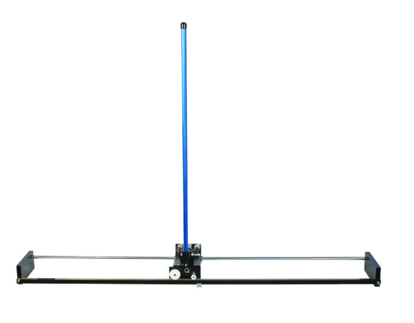
You will perform four labs in this course. The lab documents are posted on the institutional website. The experimental setup used in the lab is the inverted pendulum in the figure.
Lab 1 is an introduction to the Arduino Mega microcontroller, and its interface with motors and encoders. In this lab you will design a proportional controller stabilizing the cart in the middle of the track. In Lab 2 you will design an observer-based controller making the cart (with pendulum removed) asymptotically track a square wave reference signal. Lab 3 is simulation-based. In it, you will develop a Simulink diagram to simulate the dynamics of the pendulum on cart system, and design state feedback controllers stabilizing the unstable equilibrium of the pendulum corresponding to the inverted configuration. In Lab 4, you will adapt the results of Lab 3 and test the controller on the actual cart-pendulum experiment. In this lab you will test and compare two controllers: an output feedback stabilizer and an output feedback integral controller.
Labs are performed in groups of two or three students. You'll form lab groups at the first lab session. All labs, except the first one, require a preparation and a report
Preparation submission guidelines: Each lab document explains what preparation-related material needs to be submitted on Quercus. Each group must submit this material by 5PM, two days before their lab session. See the course calendar for the precise due date.
Report submission guidelines: Each lab document provides guidelines detailing the format to be used for the report and what needs to be included in it. There is also a description of the mark breakdown for the lab. Each lab group must submit the lab code and lab report by 5PM of the date indicated in the course calendar.
There are no make-up labs. The TA will mark down the attendance. For lab 1, there will be a penalty of 2% of the course grade for failing to attend the lab session.
| Section | Day and time | Lab 1 | Lab 2 | Lab 3 | Lab 4 |
|---|---|---|---|---|---|
| PRA0101 | Mon 15-18 | Sept 30 | Nov 4 | Nov 18 | Dec 2 |
| PRA0102 | Mon 15-18 | Sept 23 | Oct 21 | Nov 11 | Nov 25 |
Lab policies
- Lab 1 will not be graded but attendance and active participation are required. There will be a penalty of 2% of the course grade for not attending the lab.
- Labs 2-4 are marked. The grading scheme is found in the lab documents.
- We do not accept requests to manually switch a student to a different practical section. Any section switch must occur through ROSI.
- If you fail to attend a lab, your maximum grade for the lab will be 3/10.
- Labs 2-4 have a preparation. Each group must submit one preparation by 5PM, two days before their lab session (the precise due date found in the course calendar). Late submissions will receive a penalty of 1.5 points.
- It is essential that you arrive in time at the lab. Late arrivals will be subject to a penalty of 1 point.