Teaching > ECE470S
ECE470S - Robot Modelling and Control (Winter 2026)
Calendar Description
3/1.50m/1m/0.50
III,IV-AECPEBASC, III,IV-AEELEBASC,
IV-AEESCBASER,
IV-AEESCBASET,
IV-AEESCBASEZ
Classification of robot manipulators, kinematic modeling, forward and
inverse kinematics, velocity kinematics, path planning, point-to-point
trajectory planning, dynamic modeling, Euler-Lagrange equations,
inverse dynamics, joint control, computed torque control,
passivity-based control, feedback linearization.
Prerequisite: ECE311H1 or ECE356H1
Exclusion: AER525H11
Graduate Attributes
- Problem analysis:
- Demonstrate the ability to formulate and interpret a model
- Demonstrate the ability to execute solution process for an engineering program
- Investigation:
- Demonstrate the ability to use critical analysis to reach valid conclusions supported by the results of the plan
- Use of Engineering tools:
- Demonstrate ability to use discipline specific techniques, resources and engineering tools
- Show recognition of limitations of the tools used
Reference: UofT Engineering Graduate Attributes Poster
Learning Objectives
This course gives a thorough coverage of the five foundational problems of manipulator robotics:
- The forward kinematics problem: How to compute the position and orientation in space of the robot's end effector as a function of the robot's joint variables (angles or displacements of each link)
- The inverse kinematics problem: The converse of the forward kinematics problem: given a desired position and orientation of the robot's end effector, determine the corresponding (generally non-unique) joint variables.
- The motion planning problem: Using the artificial potential method, determine reference signals for the robot's joints making the robot transition between desired initial and final configurations, while avoiding obstacles.
- Robot dynamics: Using the Euler-Lagrange equations, determine the equations of motion of a robot in an algorithmic fashion.
- Robot control: Given reference signals for the joint variables of the robot originating from the solution of the motion planning problem, design feedback control loops making the robot joint variables asymptotically approach the reference signals.
Instructor
M. Maggiore
GB344
maggiore (at)
ece.utoronto.ca
Teaching Assistants
The email addresses of the TAs are obtained from the entries in the second column below by appending "@.mail.utoronto.ca" to the email ID
| Saima Ali | saiima.ali |
| Liza Babaoglu | liza.babaoglu |
| Fatima Ghadieh | fatima.ghadieh |
| Patricia Hong | patricia.hong |
| Lukasz Jagodzinski | lukasz.jagodzinski |
| Jesse Macht | jesse.macht |
| Emily Vukovich | emily.vukovich |
Lectures
Attendance will be recorded via a short in-class Quercus check-in at the beginning of each lecture. Students must submit their UofT student number during the specified time window; submissions outside this window will not be counted.
| Tue 13-14 | BA1220 |
| Wed 13-14 | GB244 |
| Fri 13-14 | GB244 |
Composition of Final Mark
| Labs | 20% |
| Quiz | 10% |
| Midterm Exam | 20% |
| Final Exam | 50% |
Textbook
Spong, Hutchinson, Vidyasagar, Robot Modeling and Control, Wiley, 2006 or alternatively, the second edition of this book, published in 2020.
Note: previous versions (pre-2006) of this text cannot be used for this course.
Additional Reference Texts
- P. Corke, Robotics, Vision and Control, Springer, 2nd ed., 2017
- J.J. Craig, Introduction to Robotics, Modeling and Control, Prentice Hall, 3rd ed., 2005
- K.M. Lynch, F.C. Park, Modern Robotics, Cambridge University Press, 2017
Course Outline
- Classification of robotic manipulators and common kinematic arrangements
- Rigid motions
- Rotations, rotational transformations, and their parametrizations
- Composition of rotations
- Homogeneous transformations
- Forward and inverse kinematics
- Kinematic chains and forward kinematics
- Denavit-Hartenberg convention
- Inverse kinematics
- Velocity kinematics
- Angular velocities; addition of angular velocities; linear velocities
- Geometric and analytical Jacobian
- Static relationship between end effector forces and joint torques
- Inverse velocity and acceleration
- Kinematic singularities
- Path planning using artificial potential fields
- Independent joint control
- Dynamics
- D'Alembert-Lagrange principle and Euler-Lagrange equations of motion
- Kinetic and potential energies of a robot
- Equations of motion of a robot
- Nonlinear control of robot manipulators
- PD control with gravity compensation
- Feedback linearization
- Adaptive passivity-based control
Calendar of deliverables
| Deliverable | Due date |
|---|---|
| Quiz | Feb 6 |
| Midterm test | Mar 5 |
The calendar above does not contain lab deliverables. The dates of these will depend on the practical section you are in. See the Assignments section of Quercus for these deadlines.
Quiz
| Date/Time | Room |
|---|---|
| Friday, February 6, 6-7PM | EX310 |
Midterm Exam
| Date/Time | Room |
|---|---|
| Thursday, March 5, 6-8PM | RW110 |
Tutorials
| Section | Day and Time | Dates |
|---|---|---|
| TUT101 | Fri 6-7PM, BA2135 | weekly starting on Jan 9 |
| TUT102 | Fri 6-7PM, BAB024 | weekly starting on Jan 9 |
Laboratories (BA3114)
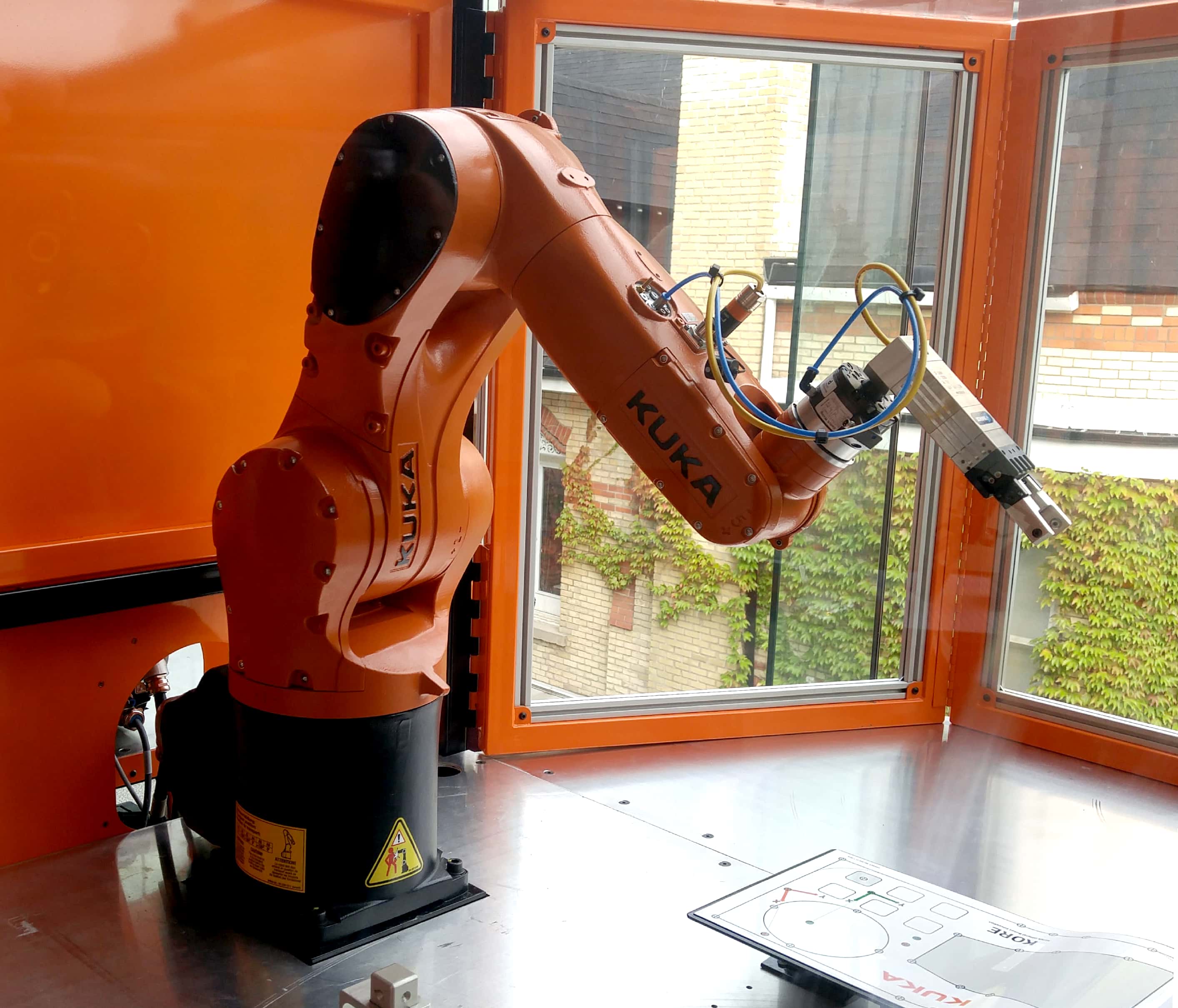
You will perform five labs in this course. The lab documents are posted on Quercus. The experimental setup used in the lab is the KUKA robot in the figure.
Lab 0 familiarizes you with the KUKA robot and safety procedures to work with it. Lab 1 is Matlab-based. In it, you'll write Matlab code implementing forward and inverse kinematics for a PUMA560 manipulator. Lab 2 is hardware-based, and it deals with the KUKA robot depicted in the figure. You will first familiarize yourself with safety procedures and learn how to manually move each of the robot axes. Then, you will adapt the code you've developed in Lab 1 to run on the actual KUKA robot. Using this adapted code, you will make the KUKA robot draw patterns on paper. Lab 3 is Matlab-based. You will write Matlab code for motion planning of a PUMA560 manipulator. Lab 4 is hardware-based. You will adapt the Lab 3 code for implementation in the actual KUKA robot. First, you'll make the robot pick up an object and drop it at a different location, while avoiding two large obstacles. Then, in a creative development phase, you'll develop your own motion planning algorithm making the KUKA robot perform more complex maneuvers.
All labs will be run in BA3114. Attendance is mandatory, and there are no make-up labs. Labs are performed in groups of two or three students. You will form groups at the beginning of Lab 0.
All labs, except lab 0, require a preparation. Each lab group submits the preparation on Quercus at least 48 hours before the beginning of the lab. After the lab is completed, each lab group submits their code, photos and videos, as applicable, on Quercus.
| Section | Day and Time | Lab 0 | Lab 1 | Lab 2 | Lab 3 | Lab 4 | |
|---|---|---|---|---|---|---|---|
| PRA0101 | Thu 15-18 | Jan 22 | Feb 5 | Feb 26 | Mar 12 | Mar 26 | |
| PRA0102 | Thu 15-18 | Jan 29 | Feb 12 | Mar 5 | Mar 19 | Apr 2 | |
| PRA0103 | Fri 9-12 | Jan 23 | Feb 6 | Feb 27 | Mar 13 | Mar 27 | |
| PRA0104 | Fri 9-12 | Jan 30 | Feb 13 | Mar 6 | Mar 20 | To be rescheduled b/c of Good Friday | |
| PRA0105 | Mon 15-18 | Jan 19 | Feb 2 | Feb 23 | Mar 9 | Mar 23 |
Lab policies
- Labs 1-4 are graded according to the following marking scheme:
- Preparation: 3 points
- Code: 5 points
- In-lab performance: 2 points.
- Attendance of Lab 0 is mandatory. Students who fail to attend it will not be given access to the hardware labs, lab 2 and 4.
- We do not accept requests to manually switch a student to a different practical section. Any section switch must occur through ROSI.
- If you fail to attend a lab, only your preparation will be graded so your maximum grade for the lab will be 3/10.
- Labs 1-4 have a preparation. Each group must submit one preparation at least 48 hours before the beginning of their lab session. Late submissions will receive a penalty of 50% of the preparation grade, i.e., 1.5 points.
- It is essential that you arrive in time at the lab. Late arrivals will be subject to a penalty of 1 point.
- Use of Generative Artificial Intelligence Tools. Students may not use artificial intelligence tools for creating computer code or solving prelabs. However, these tools may be useful when gathering information from across sources and assimilating it for understanding. The knowing use of generative artificial intelligence tools, including ChatGPT and other AI writing and coding assistants, for the completion of, or to support the completion of computer code or solution of prelabs may be considered an academic offense in this course.